A word cloud is a visual representation of common words in a text, where the more frequent words are shown in a larger font. This type of visualization helps to understand the important subjects in a text. This can be useful for identifying common issues from customers and readers.
In our example, we are creating a dataset of text from Teddy Roosevelt's "Man in the Arena" speech.
my_text_1 <- "It is not the critic who counts; not the man who points out how the strong man stumbles, or where the doer of deeds could have done them better. The credit belongs to the man who is actually in the arena, whose face is marred by dust and sweat and blood; who strives valiantly; who errs, who comes short again and again, because there is no effort without error and shortcoming; but who does actually strive to do the deeds; who knows great enthusiasms, the great devotions; who spends himself in a worthy cause; who at the best knows in the end the triumph of high achievement, and who at the worst, if he fails, at least fails while daring greatly, so that his place shall never be with those cold and timid souls who neither know victory nor defeat."
We'll open the dataset to vefiy that everything looks alright. 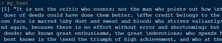
The tm package is a very commonly used package for text mining in R. In order to perform text analytics we first have to convert the data to a volatile corpus. A corpus is a collection of text documents and “volatile” means that it is stored in temporary memory.
library(tm)
my_text_1<- Corpus(VectorSource(my_text_1))
The function tm_map allows you to perform various transformations on the data. The first of these transformations will be to use content_transformer(tolower) to convert all of the text to lower case.
my_text_2<- tm_map(my_text_2, content_transformer(tolower))
The function removeNumbers removes all numbers from the text.
my_text_2<- tm_map(my_text_2, removeNumbers)
Stop words are common words such as ‘the’, ‘or’, ‘to’, ‘and’, etc. that do not add any value to a text analysis and should therefore be removed. removeWords specifies that we wish to delete certain words from our corpus. The tm_map package has a list of stop words in various languages. In the code below we are specifying that we are using stop words in English.
my_text_2<- tm_map(my_text_2, removeWords, stopwords("english"))
Finally, we can remove punctuation and extra white spaces.
my_text_2<- tm_map(my_text_2, removePunctuation)
my_text_2<- tm_map(my_text_2, stripWhitespace)
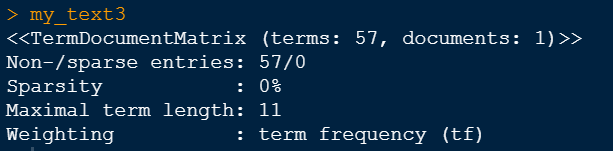
A term-document matrix describes the frequency of terms that occur in a corpus. After cleansing the data, it can be seen that our corpus has 1 document and 57 unique words.
my_text_3<- TermDocumentMatrix(my_text_2)
my_text_3
The as.matrix function puts the data into a matrix form. Since our corpus was 1 document and 57 unique words, the matrix will be 1 by 57.
my_text_4<- as.matrix(my_text_3)
my_text_4
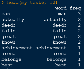
The rowSums function will sum the rows in the matrix and sort will sort the values highest to lowest. Putting the data into a data frame will make it easier to read. The most frequent words can be seen in the figure below. It is at this point that we can go back to a previous step and exclude words if we see anything here that does not seem valuable to the analysis.
my_text_5<- sort(rowSums(my_text_4),decreasing=TRUE)
my_text_6<- data.frame(word= names(my_text_5),freq=my_text_5)
head(my_text_6, 10)
Although the results above are adequate for our analysis it is helpful to present these in a colorful, visual style. Below is the code for the word cloud itself. If you set the seed to any number, every time you run the code the output will look exactly the same. If you do not do this, every time you run the code, the words in the word cloud will be in different positions. The min.freq= 1 setting means that we are only returning words that showed up at least once. If we had a bigger dataset, you would want to set this to a larger number. You can use trial and error with the scale setting to make sure that all the words fit on the output. If all the words do not fit because the font is too big, an error message will show up letting you know that words were left out.
library(wordcloud)
set.seed(123)
wordcloud(words= my_text6$word, freq= my_text6$freq,
min.freq= 1, scale=c(3,0.2), max.words=30,
random.order=FALSE, rot.per=0.35, colors=brewer.pal(8, "Dark2"))
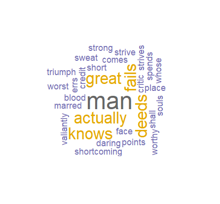
As can be seen in the output, the word that stands out the most is "man" with others like "great", "fails", etc. and second most common. Again if we had a larger text file, the distribution would vary greater and the output would be more colorful, but this word cloud still gives us a great visual to explain the text.