Language Overview
SQL which stands for “Structured Query Language” is a language used to retrieve and manage data from relational databases. It was created by Donald Chamberlin and Raymond Boyce in the 1970s for IBM and is based off of the concept of relational models conceived by Edgar Codd. In the mid-1980s, SQL had become an ANSI (American National Standards Institute) standard. Today SQL is used extensively; from reporting to websites, this is the language that is behind much of the data we see.
Being a declarative language, you are telling the database what data you want. Querying is one of the most important functions of SQL. However, it is much more than just simply pulling data from a database. SQL can be used to specify exactly what data you want to retrieve, update databases and tables, create your own tables and perform complex calculations.
Not all SQL code is universal. There are variations of SQL such as SQL PL, T-SQL (MS Access), SQL/PSM (MySQL), PL/SQL (Oracle), and SPL (Teradata). Hive, which is a language used for big data platforms such as Hadoop is SQL-like. Although there can be subtle differences in syntax depending on the program you are using, basic statements like SELECT, FROM, WHERE, CASE, CREATE TABLE, DROP TABLE, INSERT INTO, DELETE FROM, and JOIN are homogeneous across all platforms.
At the most basic level, you select particular columns from a table that fit a certain criteria (a WHERE statement). Inner joins, full outer joins, left joins, right joins are some of the functions that you can use to connect different tables together. As you become more familiar with the language, it will be easier to write your code in a way that will return the data in a timely and efficient manner.
SQL Basics
There are aspects of SQL that can be quite complex, but the overall basics of the language can be summed up by three basic operations: SELECT, FROM, and WHERE. The SELECT statement is used to specify which fields of the table you would like to retrieve. The FROM statement denotes the table or tables in which the fields reside. The WHERE statement gives specific criteria for the values you want returned. Within the WHERE statement, operators such as =, <, >, <=, >=, <>, BETWEEN, OR, AND, IN, and NOT IN are used to denote the criteria to retrieve specific data.
Let’s start off using a table called sales_tbl that contains sales transaction information. The code below shows how to retrieve every field and every row in the table without any specific criteria. The asterisk in the statement means that you want to pull back every field in the table, otherwise you would specify each field individually that you wish to return.
select * from retail_db.sales_tbl;
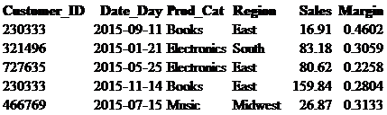
The results in the figure above show every field and every row, but what if we only want to see Customer_ID, Date_Day, and Prod_Cat for the Electronics category for transactions that occurred between January and May. As seen in the code below, the WHERE statement allows us to do this. Notice that non-numeric fields are put in single quotes. The date field needs to be put in the format of ‘yyyy-mm-dd’ and requires a BETWEEN and AND statement to specify the range of dates. As can be seen in the output below, there are two values returned that fit our criteria.
select Customer_ID, Date_Day, Prod_Cat
from retail_db.sales_tbl
where Prod_Cat= ‘Electronics’
and Date_Day between ‘2015-01-01’ and ‘2015-05-31’;
Let’s now retrieve instances where a customer’s sales were greater than $50. The ORDER statement sorts the values of a particular field in ascending or descending order. The default order is ascending, but if you wanted to return values in descending order you would use the DESC operator after the field name in the ORDER statement.
select *
from retail_db.sales_tbl
where Sales > 50
order by Sales desc ;
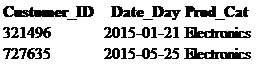
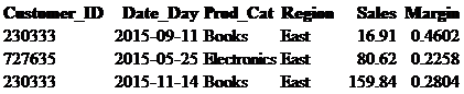
Within the WHERE statement, another operator used to select specific criteria is IN. Earlier we retrieved data by using the equal sign. This is fine if you have one value in your criteria, but the IN operator can be used when you have multiple values.
select *
from retail_db.sales_tbl
where Customer_ID in (727635,230333);
What if we want to see what product categories these customers shopped in. If we were to do a basic SELECT statement as we did above, it would give us the result seen in the table below.
select Prod_Cat
from retail_db.sales_tbl
where Customer_ID in (727635,230333);

Notice how the ‘Books’ category is in there twice; since we are only interested in seeing how many distinctive categories there are, the DISTINCT operator can be used to return unique values.
select distinct Prod_Cat
from retail_db.sales_tbl
where Customer_ID in (727635,230333);

Variable Transformation
Rarely do datasets have all of the variables that we need, and often they are not in the format we would like. To create a good analysis, it is imperative that we are using exactly the data we need to reach our outcome. Creating and transforming variables are therefore essential in any analysis.
The first step is to make sure that the variables you are using are in the desired format. The CAST function is used to transform variables from one data type to another. As was mentioned in a previous chapter, there are many different data types that exist, so it is important to familiarize yourself with them.
In our table sales_tbl, the variable customer_id was assigned as an integer. If we wanted to transform this into a decimal, the CAST function as seen in the code below would be used. Keep in mind that different SQL querying platforms use different syntax. For example an integer can be denoted as INTEGER, INT, or SIGNED.
Notice that after the operation we have used the code as customer_id_new, this is called an alias and is the name of the column we just created. If we did not state an alias after our operation, the column name would have been shown as cast(customer_id as decimal (10,2)) instead of customer_id_new.
select cast(customer_id as decimal (10,2)) as customer_id_new
from retail_db.sales_tbl ;
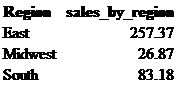
As was mentioned, some key statements are FROM, WHERE, AND, and OR. These help to define your initial population, but there are many more functions that can be used to transform the data. One of the most important and frequently used of these is the SUM function which is used to sum numerical data. The SUM function needs to be used in conjunction with the GROUP BY statement for all of the other variables not being manipulated.
Let’s say that we want to use our sales_tbl table to calculate sales dollars by region. The only variables we care about are Region and Sales where Region is categorical and Sales is numeric. The code would be as follows:
select Region, sum(Sales) as sales_by_region
from retail_db.sales_tbl
group by Region ;
The COUNT function is also a very widely used function and is applied when you want to know the quantity of a particular field. For example, if we wanted to know how many customers there are in our table, we can do a count on Customer_ID. Remember how we discussed before that using the distinct function will return unique values. If in the code below we were to not include distinct, the result would be 5. Using distinct returns a number of 4 which tells us that there are 4 unique customer IDs in this table.
select count(distinct Customer_ID)as nbr_customers
from retail_db.sales_tbl ;
Excluding the distinct statement is necessary some times. For example, if we wanted to know how many total transactions there are, we would want to count every row in the table. When retrieving data, it is important to really think logically about how you want the data returned.
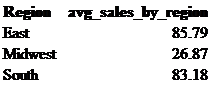
There are many additional functions that can be used on numerical data: addition, subtraction, averages, division, multiplication, etc. Instead of returning total sales by region as in Figure 5.1, we may want to see what the average sales are; this can be done using avg. Additionally, if we cast this as a decimal, the average sales will be returned with two decimal places.
select Region,
cast(avg(Sales)as decimal (10,2)) as avg_sales_by_region
from retail_db.sales_tbl
group by Region;
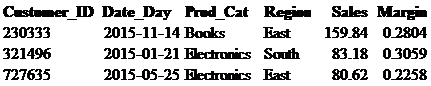
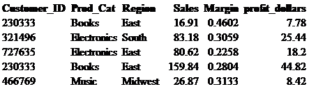
We know what the sales and margin are for each customer, but what if we want to know what total profit dollars are even though this field does not exist? In this case we would simply take Sales times Margin and create a new field called profit_dollars. Again, use the cast function so that the returned values are at two decimal places.
select Customer_ID, Prod_Cat, Region, Sales, Margin,
cast((Sales * Margin) as decimal (10,2)) as profit_dollars
from retail_db.sales_tbl ;
The CREATE TABLE function can allow you to create a permanent table in a database. However, some database administrators will prohibit you from using this function and in certain cases it is inefficient to use CREATE TABLE when you are using it as one piece in a multi-layer chunk of code. A common practice is to use what is called a subquery or nested query. A subquery is a temporary table nested inside another query.
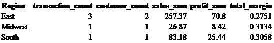
We may want to see how many transactions, unique customers, sales, profit dollars, and margin there are per region. The bolded code below is the subquery. As good practice subqueries are generally indented so that it is easy to see what is a subquery and what is not. You will notice that we have put at T1 at the end of this. Similar to the aliases we use when creating new fields, subqueries need a designated table name. Although this table name can be anything you want, standardized names like T1, T2, etc. make it easy to follow. In a bit we will be talking about joining tables; this is another situation where you need to create aliases for each of your tables.
select Region, count(Customer_ID)as transaction_count, count(distinct Customer_ID)as customer_count,
sum(Sales) as sales_sum, sum(profit_dollars) as profit_sum,
cast(sum(profit_dollars)/sum(Sales)as decimal (10,4)) as total_margin
from
(select Customer_ID, Date_Day, Prod_Cat, Region, Sales, Margin,
cast((Sales * Margin) as decimal (10,2)) as profit_dollars
from retail_db.sales_tbl
group by Customer_ID, Date_Day, Prod_Cat, Region) T1
group by Region;
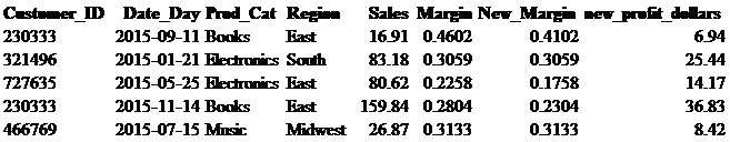
What if there was a scenario where the margins for our stores in the East region had to be adjusted by 5%. How would we perform a calculation like we did above, but for only rows of data that fit specific criteria? A CASE statement is similar to IF, THEN, ELSE statements that are common among other programing languages except that CASE statements have the structure of CASE WHEN, THEN, ELSE. In the code below, you can see the CASE statement in bold. We are saying that when Region is equal to ‘East’ then take Margin minus .05; if Region is anything other than ‘East’ then return the current value in the Margin field. This new field New_Margin in the subquery is then being used to calculate new_profit_dollars.
select Customer_ID, Date_Day, Prod_Cat, Region, Sales, Margin, New_Margin,
cast((Sales * New_Margin) as decimal (10,2)) as new_profit_dollars
from
(select Customer_ID, Date_Day, Prod_Cat, Region, Sales, Margin,
case when Region =’East’ then Margin -.05 else Margin end as New_Margin
from retail_db.sales_tbl) T1 ;